COURSES: Some Special Skills of Microsoft Excel for Accountants

If you are an accountant, one of the most important skills for you to master is Microsoft Excel, period.
Why I'm Saying This?
Well, financial data is what you deal with as an accountant, and you need to be good at managing and analyzing data, right?
And Microsoft Excel is the tool you need.

To get started with it, you can learn:

Introduction to Excel
Excel Tips
Excel Functions with Examples

BUT.

You are an accounting professional, so you also need to learn all those specific things which can help you to thrive in our work.

Let me tell you that this is the most comprehensive guide which you can find on the internet to help you to be a better accountant.

So let's get started.

1. Keyboard Shortcuts for Accountants

No matter is you are an accountant, finance professional, or in some other profession, using keyboard shortcuts can help you to save a lot of time.

Ctrl + Shift + $ (Applies the currency format)
Ctrl + ! (Open the format option dialog box)
Control + T (Applies the Excel table to the selected data.)
Alt + = (Sums the values from the upper or left cells)
Alt H W (Applies the wrap text to the selected cell)
Alt W F F (Applies the freeze pane from the selected data)
Alt N V (Insert a pivot table with the selected data)
Alt + F11 (Insert a chart from the selected data)
Control + Shift + D (Apply filters to the data)
Alt A M (Remove Duplicates)

Here are my few tips for every accountant about keyboard Shortcuts.

Replace your 10 most used options with keyboard shortcuts.
Try to locate shortcut keys by pressing the ALT key.

2. Power Of Paste Special

One of the options which you need to learn is PASTE SPECIAL. With it, you can do a lot of things other than a normal paste.

To open the paste special option, you need to go to the Home Tab → Clipboard → Paste Special or you can also use the Shortcut Key Control + Alt + V.

Once you open it you can see there are more than 16 options to use, but let me share the most useful options which you need to learn:

Values: It only pastes values, ignoring formulas and formatting from the source cell and best to use if you want to Convert formulas into values.

Foumulas: It only pastes formulas, insteaad of values and best to use if you want to use apply formulas.

Formats: It copies and pastes the formatting, ignoring values and formulas from the source cell (Quick tip: Format Painter).

Column Width: It only applies the column width to the destination column, ignoring the rest.

Operations: With this option, you can perform simple (multiply, divide, subtract and addition calculations

3. Sort Data Like A Pro

In Excel, there are multiple ways to sort data. When you open the sort dialog box (Data Tab → Sort & Filter → Sort), you can add a level to sort.

Imagine if you want to sort the below data using the first_name column, you need to add a sorting level for this:

1. First of all, select the column from the "Sort By".

2. After that, in "Sort On", select "Cell Values".

3. In the end, in "Order", A to Z.

Once you click OK, You'll get the data sorted like below:

Well, this was the basic way to sort data which is mostly used, but apart from that, there are some advanced sorting options that you can use.

1. Sort On

From the "Sort On" drop-down, you can select the option to sort with font color, cell color, or conditional formatting.

So, if you select the cell color, it gives you the further option to show it on the top or at the bottom after sorting.

2. Custom List

You can also create a custom list of sorting values. Imagine you have a list of names and you want all the names in a particular order, you can create a custom list for that.

3. Sorting Column

By default, when you use sort option it sort by rows but there's an option which helps you to sort data by column. Open the "Options" and tick mark the "Sort Left to Right"

4. Advanced Options to Filter Data

Excel filter is fast and powerful. It gives different ways to sort data from a column. When you open a filter you can see there are a lot of options that you can use.

Below I have listed the most useful options which you can use:

1. Filter by Color

So if you have cell color, font color, or even applied conditional formatting, you can filter all those cells as well.

2. Custom Filter

With custom filter, you can filter using conditions, partial match, wildcard characters, much more.

3. Data Filters

If you have dates in the column, you can use date filters to filter them in different ways, like weeks, months, and years.

4. Search Box

With the search box, you can filter values in a flash. You just need to type the value and hit enter.

5. Apply Excel Table to the Data Every Time

If I have to give one tip Excel, I'd like to say "Use Excel Tables Every Time". Why I'm saying this? Well, there's a hige benefit to using Excel tables.

To apply Excel table to data you can go to Insert Excel Table or you can also use the Shortcut Key Control + T.

When you refer to this data in a table, every time you update this data you need to change the reference

why? Because the range address of the data changes every time you update it.

The best example I can tell you is about using a table while creating a pivot table, you can use a table to update source range automatically for a pivot table.

6. Conditional Formatting for Better Presentation

Conditional Formatting is smart formatting. It helps you to format data based on a condition or a logic and it helps you to present your data in a batter way and also gives you quick insights.

To access CF, you need to go to the Home Tab → Style → Conditional Formatting.

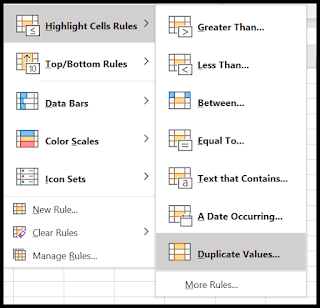
Let's say you want to highlight duplicate values, with the conditional formatting you can do this with a single click. Highlight Cell Rules → Duplicate Values.

Or if you want to highlight the top 10 values, there is an option in conditional formatting called "Top Bottom Rules" which you can use.

In this same way, you can also apply data bars, color scales, or icons sets on your data.

And if you want to create a custom rule to apply CF, click on the "New Rule" and you'll get a dialog box to create a new rule to apply conditional formatting.

7. Advanced Find and Replace for Smart Users

Apart from normal find and replace there are a few advanced options in Excel to use find and replace.

For thi, you need to click on the "Options" button and you'll get a bunch of options down the line. Below I have described them:

1. Within: You can select area fo the value. You can select between the active worksheet and the whole workbook.

2. Search: Search through rows or columns.

3. Look in: Look in formulas, values, comments, and notes (This option only works find not with find and replace).

4. MatchCase: Find and replace a value with a case sensitive search.

5. Match Entire Content: Match values from the entire value of a cell with the searchedvalue.

6. Format: With this option, you can search a cell based on its formatting. You can soeify the formatting or you can use a selection tool to select it from a cell.

8. GO TO Special for Fast Data Selection

With GO TO Special, ou can select specific cells just with a single click.

Once you this, you can see the list of types of cells and objects.

Imagine if you want to select all the cells where you have formulas and thode formulas show an error.

You just need to select the formula and tick mark only errors and click OK and all the cells with formulas with errors will get selected.

9. Use Sparklines for Tiny Charts

As an accountant, you need to deal with a lot of financial data in tabular form and sometimes for the end users, these kinds of data take longer to understand.

But with sparklines, you can make it easily igestible by creating tiny charts. In the below example, I have product-wise and year wise data and at the end of the rows, I have small charts which I have added by using sparklines.

Basically, there are three different types of sparklines which you can use:

Line
Column
Win/Loss

To add a sparkline you simply need (Insert Tab → Sparklines) and select the type which you want to insert.

Once you click on the type, you'll get a dialog box where you need to select the data range and then you need to specify destination the cell for the sparkline.

Once you insert it, there are multiple ways to customize it. Simply click on the cell and go to the Sparkline.

You can add and remove markers add high-low points.
You can change the color of the marker and the line.
You can also change the type of Sparkline in your work.

10. Data Analysis With Pivot Table

A pivot table is the most important tool when it comes to data analysis in Excel. You can create a pivot table to create instant financial reports and account summaries of a large set of data.

Well, creating a pivot table is easy.

You need to have source data just like I have in the below example, but make sure there shouldn't be any blank row or column

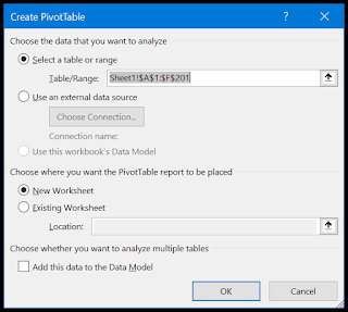
Now, go to the Insert Tab and click on the insert pivot table.

It will show you a dialog box to define the source data range but as you have already selected the data it takes it automatically.

Once you click OK, you will have sidebar just like below where you can define the rows, columns, and values for the pivot table. You can simply drag and drop.
So now, add "Age" to the rows, "Education" to the column, and "First Name" to the values.